Project Overview

Precipitation is the driver of terrestrial hydrology. Extreme precipitation is either the primary or secondary cause of many natural hazards such as floods, avalanches and landslides. The societal impact of precipitation is significant in the UK. Mitigation techniques, such as flood defences and evacuations, can minimise damage and cost during these events (Baker et al., 2016; Marsh and Hannaford, 2007). In order to enable sufficient time for relevant authorities, businesses and individuals to take action, accurate precipitation forecasts and warnings are necessary well in advance of the event itself. There are many instruments and various methods of measuring precipitation, such as tipping bucket rain gauges, disdrometers and weather radar. During the past few decades, it has become clear that weather radar is the most feasible technology which can provide quantitative precipitation estimation (QPE) with high resolution in both the temporal and spacial scales necessary for accurate hydrological predictions (Berne and Krajewski, 2013). Furthermore, radar has the unique ability to monitor rapidly developing events as well as to track the speed and direction of movement of precipitation systems (Fabry, 2015). Therefore, accurate QPEs rely principally on stable hardware components and an accurate sensitivity calibration (Harrison et al., 2000). Regardless of hardware issues, several other phenomena (icing, wind shear, severe storms, etc.) can affect radar estimates of precipitation rate (Beard and Robert, 1990). Often these phenomena, while being a hindrance for deriving precipitation rates at the surface, are useful in revealing microphysical processes inside clouds.

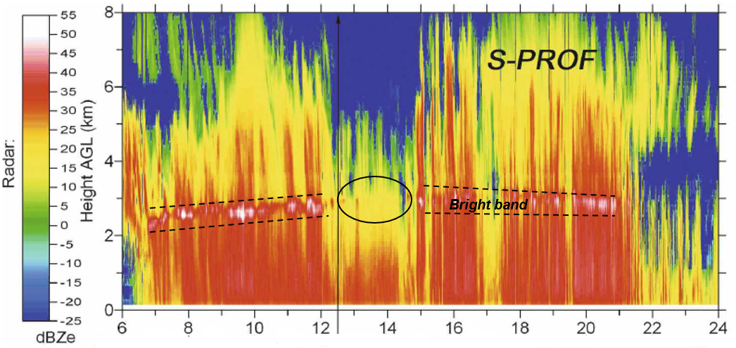
In radar data, the freezing level (0°C isotherm in the atmosphere) generally appears as a region of enhanced reflectivity at a relatively constant altitude, known as the bright band (see Figure 1) (Illingworth and Thompson, 2011). This occurs as ice crystals melt and become coated in liquid exterior surface, which the radar observes with the same reflectivity as a very large raindrop. Hence, the melting snow has larger reflectivity than both the snow above and the rain below. However, there are occasions when the bright band is absent (see Figure 1), but precipitation still goes through a process of ice nucleation and subsequent melting before it reaches the surface. Although the underlying reason why the bright band is occasionally absent is still unknown, Martner et al. (2008) suggested that there is a “statistically significant” (P-value of 0.01) difference in RR and DSD (drop size distribution) for periods with and without a radar bright band. Martner et al. (2008) compared data from the S-PROF radar and a Joss-Waldvogel disdrometer (JWD) for a period of 3 months at Cazadero and Bodega Bay, California. Approximately half of the rainfall data could be classified as occurring during periods with observed radar bright bands (BB) and half during periods where there was no bright band (NBB) observed. In these regions, NBB rainfall contributed significantly to the total winter season rainfall and to potentially flooding precipitation at times. Therefore, the difference in precipitation with and without the BB should be considered while estimating rainfall.

Many studies have found that the BB could lead to large overestimates if left uncorrected (Villarini and Krajewski, 2010). Hence, there are studies talking about the correction or detection for the BB and many government radar networks have applied correction to the enhanced reflectivity factor, e.g. the U.K. Met Office (Harrison et al., 2000) and the Météo-France (Tabary et al., 2007). As for the NBB rain, although some studies, such as Martner et al. (2008) and Mastrov et al. (2016), suggested it should be categorised as a different rain type in stratiform precipitation, currently no government radar network has considered such difference. Hence, when converting measured radar reflectivity factor (Z) to precipitation rate (R) during stratiform precipitation, only one Z-R relationship is used in the U.K. Met Office:

which is calculated from the raindrop size distribution indicated by Marshall and Palmer (1948). D is the diameter of raindrop and N(D)dD is the number of scatterers per unit volume with diameters in dD. N(D) is the DSD for raindrops.

The results in Martner et al. (2008) are not sufficiently representative – the authors did not give the specific difference for the BB and NBB precipitation, and they only analysed a 3-month dataset manually. Therefore, the objectives of this project are:

1. Deduce an algorithm in Python to identify BB and NBB during precipitation.
2. Identify the microphysical difference for the BB and NBB precipitation by comparing the Copernicus radar data with the DiVeN disdrometer data (at CFARR). Examine whether such difference in RR and DSD is similar to the one suggested by Martner et al. (2008).
3. Assess the impact of BB/NBB rainfall on climatology using the identification algorithm.
4. Calculate whether the accuracy of QPEs by radar can be improved after applying the relationship above.