Initial Algorithms
Current results are produced based on a case study for data on 12th March 2017.
Algorithm Using Radar Reflectivity Factor ($dBZ$)
The following results are produced using this script: [identify_BB_VPR.py].
A significant bright band signature does not always appear in the VPR. Hence, simply analysing VPR could not produce ideal results. The radar reflectivity factor commonly used is the logarithmic scale reflectivity factor in units of decibels ($dB$) while the true radar reflectivity factor is in units of ${\rm mm}^6 \cdot m^{-3}$. The relationship between the reflectivity factor in decibels ($dBZ$) and the (linear) reflectivity factor ($Z_{linear}$) is that:
As shown in Figure 4, $Z_{linear}$ is much more sensitive to the bright band than $dBZ$. Therefore, instead of using $dBZ$, this algorithm uses $Z_{linear}$ to identify the bright band. Some literature, e.g. Cha et al. (2009), suggested that the first derivative of the reflectivity factor is helpful for the bright band identification. Thus, analysing the first derivative of $Z_{linear}$ is another method used in this project. This method would recognise the bright band by searching for the location of the maximum change in the vertical profile (see Figure 4(c)). In addition, the second derivative is introduced into these two methods to eliminate some noise. Because, mathematically, the smallest second derivative should be located at where the $Z_{linear}$ is at its maximum and where the first derivative changes the most, vice versa.
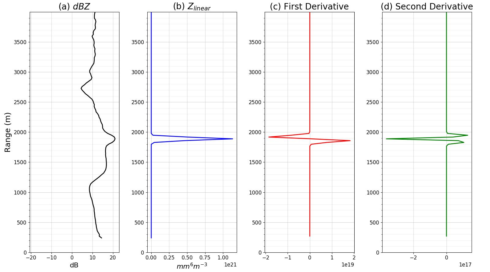
Figure 4: Vertical profiles of $dBZ$ (a), $Z_{linear}$ (b), first derivative (c) and second derivative (d) in an ideal case on 12th March 2017 at CFARR. The bright band is located at approximately 2000 m.
In order to achieve these methods by programming, both the first derivative and the second derivative should be calculated numerically. Using the finite difference, the first derivative at a point $x$ can be expressed as:
where $h$ is the radar range (height) interval. Note that the central difference is used in order to avoid shifts in data grids. The range interval of Copernicus radar is 30 m. The second derivative at a point $x$ can be expressed as:
A 750-m check is also used in these sub-algorithms. The algorithms check the vertical profiles of $Z_{linear}$ and $\frac{dZ}{dh}$ every 750 m from the highest range to the lowest and mark the largest peaks at the highest range. By doing so, some noise could be eliminated, e.g. when the rain below the bright band has the same reflectivity as the bright band, the algorithms will only mark the bright band. 750-m is the bright band width assumed. Kitchen et al. (1994) indicated that the typical width of the bright band is around 700 m, while the range interval of Copernicus radar is 30 m (700$\div$30=23.333$\ldots$). In addition, as Emory et al. (2014) suggested that the bright band thickness may change with the precipitation intensity, 750 m may be a good choice when precipitation is intense. Figure 5 shows the bright band identified by the aforementioned sub-algorithms.

Figure 5: Bright band locations marked by two sub-algorithms. The bright band marked by $Z_{linear}$ algorithm is shown as triangles. The bright band marked by the first derivative algorithm is shown as crosses.
The results produced by these two sub-algorithms generally agree with each other. Most parts of the bright band are marked correctly, but several other locations that are not the bright band are also marked. The worst part of these results is that there are some marks below the bright band and close to the ground. This is due to heavy rainfall. When it was raining heavily, the reflectivity below the bright band could be much higher than the bright band itself. As shown in Figure 6, $Z_{linear}$ is more sensitive than $dBZ$ that $Z_{linear}$ would only peak near the lower ranges due to intense precipitation. The bright band signature is relatively weak, but still visible in the vertical profile of $dBZ$. Hence, the reliability of $Z_{linear}$ varies in different cases.
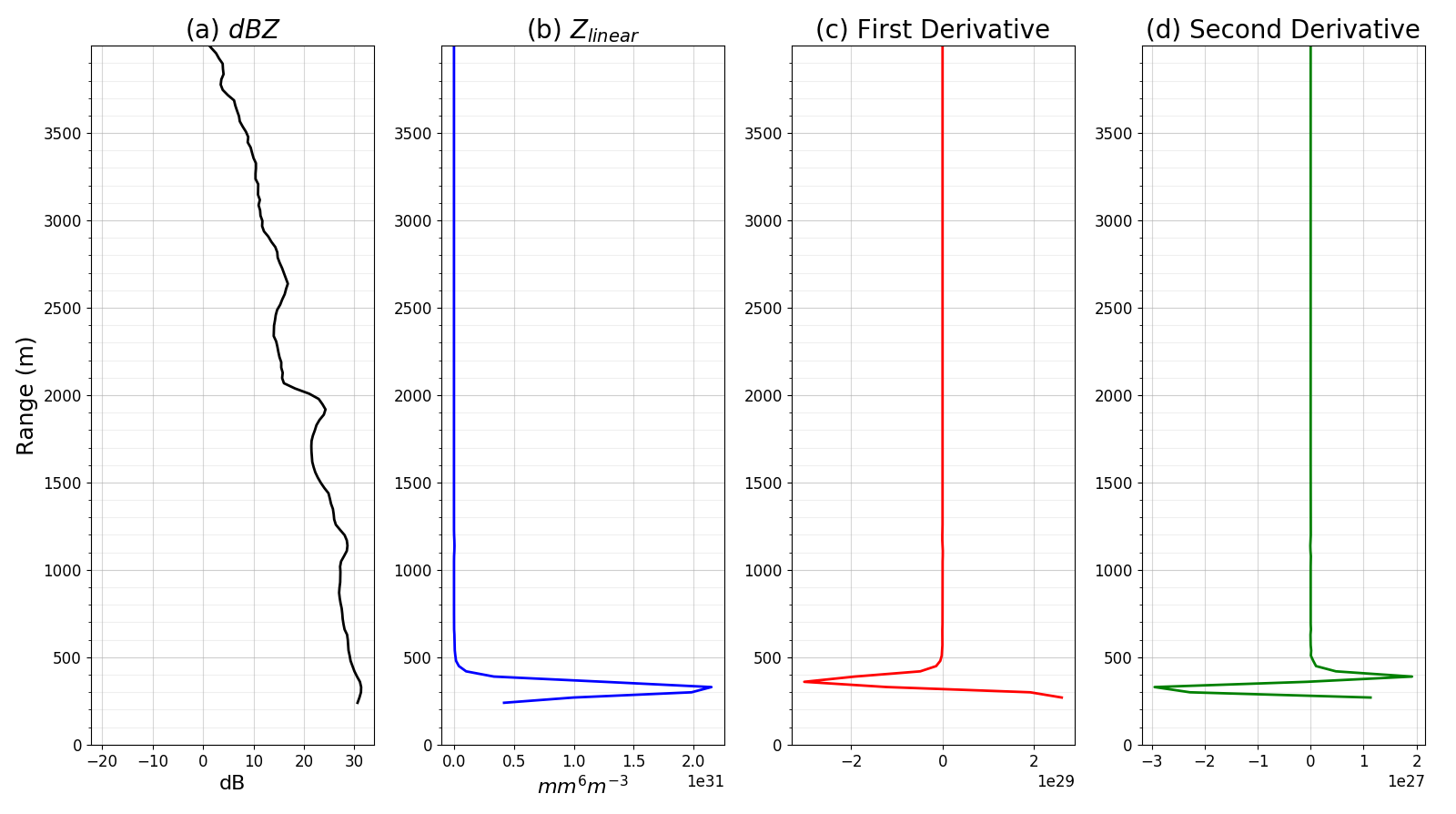
Figure 6: Vertical profiles of $dBZ$ (a), $Z_{linear}$ (b), first derivative (c) and second derivative (d) during intense precipitation period on 12th March 2017 at CFARR. The bright band is located at approximately 2000 m. Except for $dBZ$, all the variables failed to show the bright band signature.
Algorithm Using Doppler Velocity ($v$)
The following results are produced using this script: [identify_BB_Vel.py].
The fall velocity of a precipitation particle is changing corresponding to its size (Gunn and Kinzer, 1949). Nevertheless, the fall velocity for raindrops is generally larger than the fall velocity for snow particles. A vertical profile of $v$ during a bright band event is shown in Figure 7. The following flow diagram (Figure 8) shows how this “Velocity Algorithm” works. In this algorithm, particles with velocities between $0.5\ m \cdot s^{-1}$ and $1.5\ m \cdot s^{-1}$ are categorised as snow, and the lowest range of this velocity category is marked as the bright band top (BBT) – where the melting begins. Meanwhile, particles with velocities larger than $3.5\ m \cdot s^{-1}$ are classified as rain, and the highest range of that is the bright band bottom (BBB) – where the snow has almost totally melt. Finally, if the distance between BBB and BBT is within 750 m (according to Kitchen et al. (1994)), then there should be a bright band.
Please note that the thresholds here are set based on the empirical Gunn and Kinzer curve and hence are still rough.
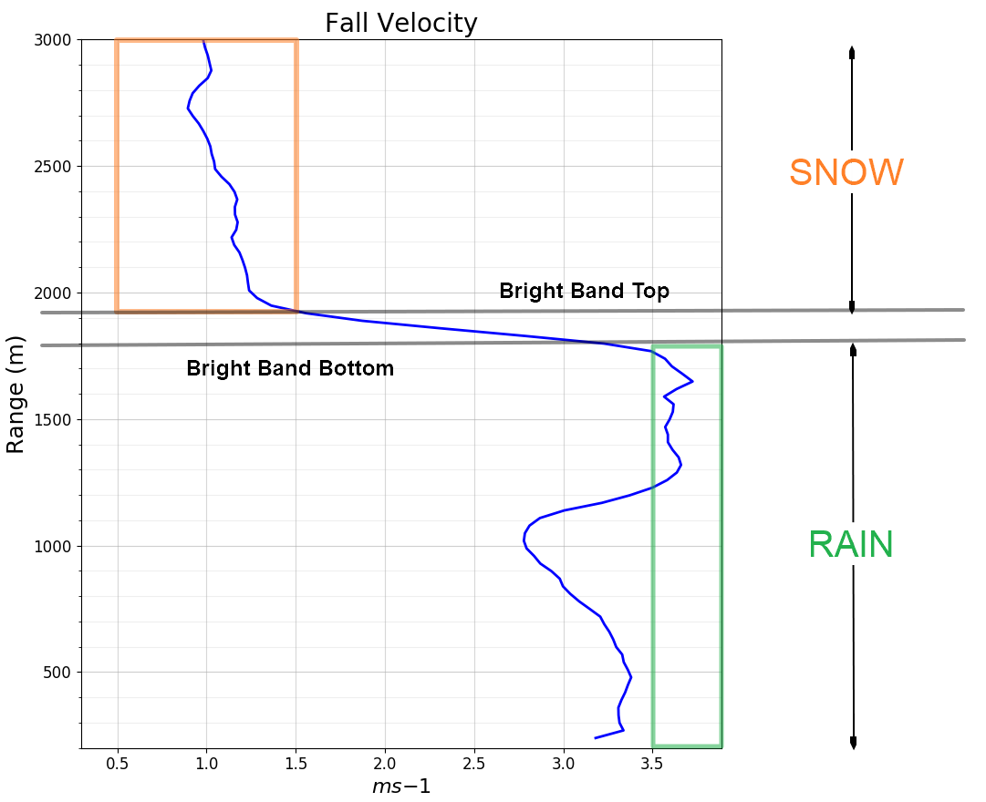
Figure 7: Configuration of the “Velocity Algorithm”. The blue curve shows the vertical profile of $v$ during bright band precipitation.
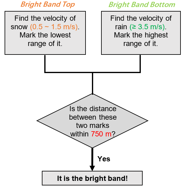
Figure 8: Simple flow diagram showing how the Velocity Algorithm is working in a Python script.
The BBT and BBB identified by this algorithm are shown below. Compared with “VPR Algorithm”, this "Velocity Algorithm" is not affected by the precipitation intensity. It shows better and more consistent results. One issue is that this method could be influenced by updrafts and downdrafts. Thus, it cannot detect the bright band location very accurately. Fixing this issue would be very complicated and may not be accomplished in this one-year MRes programme. Hence, an imporved algorithm is built.

Figure 9: The bright band identified by the “Velocity Algorithm”. Circles are the BBT location. Crosses are the BBB location.
Combined Algorithm
The following results are produced using this script: [identify_BB_combined.py].
Because neither the VPR Algorithm nor the Velocity Algorithm can produce ideal results, but they both could mark the correct bright band location in some cases, this “Combined Algorithm” then aims to identify the bright band by combining the advantages of both these algorithms.
On the one hand, apart from the effect due to updrafts/downdrafts, the Velocity Algorithm performs well in detecting the bright band, and it would not have misdetection of the bright band during intense precipitation period. On the other hand, the VPR Algorithm is not reliable during heavy rain but is not affected by those air currents motions. Hence, in this Combined Algorithm, the Velocity Algorithm is used in the first place. Then, this algorithm aims to determine whether there is a $Z_{linear}$ peak or a maximum change in $\frac {dZ}{dh}$ (the first derivative of $Z_{linear}$) profile within the area marked by the Velocity Algorithm. The flow diagram (Figure 10) and the results (Figure 11) of the Combined Algorithm are shown below.
Although the two sub-algorithms used in the VPR Algorithm agree with each other very well, both the $Z_{linear}$ method and the $\frac {dZ}{dh}$ method sometimes failed to mark the bright band. This is due to the pre-existing issue – intense precipitation. However, the results are still much better than those produced by the other two algorithms.
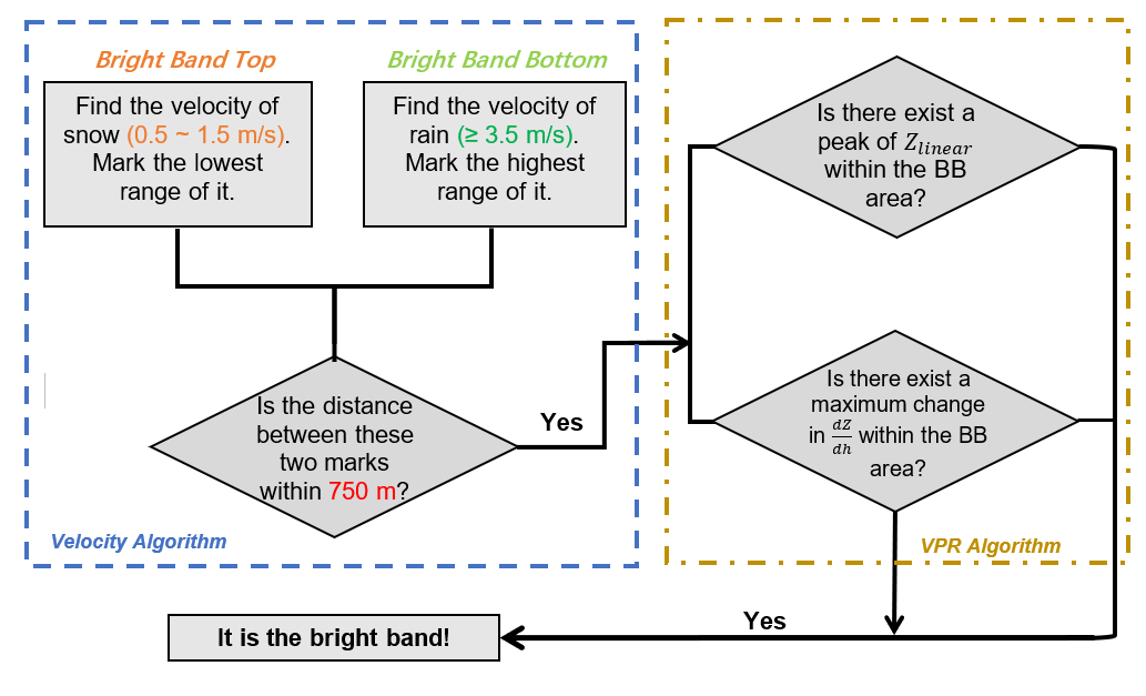
Figure 10: Simple flow diagram showing how the Combined Algorithm combines the VPR Algorithm with the Velocity Algorithm.

Figure 11: Bright band locations marked by two sub-algorithms in the Combined Algorithm. The bright band marked by $Z_{linear}$ algorithm is shown as triangles. The bright band marked by the first derivative algorithm is shown as crosses.
It is worth to point out that between 4:00 and 6:00 in Figure 11, there is a bright band, but it is relatively very weak and hence less visible. All the aforementioned algorithms failed to detect it. Figure 12 shows vertical profiles of reflectivity factor parameters and the Doppler velocity. The bright band signature can be observed, but whether this weak bright band was occurring during precipitation or not should be checked. Hence, the comparison between the Copernicus radar data and the disdrometer data have been made (described in the disdrometer section).
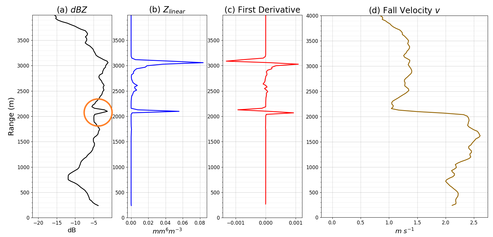
Figure 12: Vertical profiles of $dBZ$ (a), $Z_{lienar}$ (b), $\frac {dZ}{dh}$ (c), and the fall velocity ($v$) (d) during a weak bright band case. The bright band signature can be found near 2000 m in $dBZ$ profile (pointed out by the orange circle), but linear reflectivity factor parameters failed to show this as the largest peak. There existed hanges in the fall velocity, but the velocity below the bright band is smaller than the threshold ($3.5\ m\cdot s^{-1}$) set. Note that values of all these parameters are much smaller than those in a stronger bright band case.