Ongoing Algorithm
The following results are produced using this script: [identify_BB_strength.py].
If there exists any correlation between bright band strength and precipitation intensity, then there are two principal issues to be addressed. On the one hand, an identification algorithm that can recognise weak bright band correctly is required. On the other hand, the algorithm should be able to measure the bright band strength programmatically.
Adjusting thresholds set in the Velocity Algorithm is not an ideal method. Although the presence/absence of the bright band is correctly detected by this algorithm, the bright band location identified is still affected by updrafts/downdrafts. As the bright band is not always where the $Z_{linear}$ peaks, both the VPR Algorithm and the Combined Algorithm could fail to detect the bright band in some cases. Therefore, the current idea is to calculate the rate of change of the Doppler velocity, namely, the first (central) derivative. The bright band location should be where the first derivative is of its minimum (the rate of change is the largest) because the fall velocity of precipitation generally decreases with respect to height.
In this algorithm, the velocity threshold for liquid precipitation is changed from $>3.5\ m \cdot s^{-1}$ to $>2.5\ m \cdot s^{-1}$ so that both weak and strong bright bands could be identified. The first (central) derivative would only be calculated when the Velocity Algorithm identified the bright band.
The range interval of Copernicus radar is 30 m, and there are 480 pixels in the range axis. If the first (central) derivative of the velocity is calculated pixel by pixel, then the results would be very noisy, even though they are not affected by updrafts/downdrafts (as shown in Figure 14a). According to vertical profiles shown in Figure 15, the data are not continuous near the cloud top (above 4000 m in this case) and hence the first derivative would be higher there. In order to eliminate the noise, the range interval that the derivative is calculated should be adjusted. In the pixel-by-pixel central difference calculation, the total range is 60 m (3 pixels). Hence, a series of multiples of 60 were tested, e.g. 120 m, 180 m, 240 m, etc., to find the optimal interval. Currently, the optimal interval is 360 m. Corresponding results are shown in Figure 14b. In order for comparison, results with an interval of 660 m are shown in Figure 14c. Compared with 60-m and 660-m results, the 360-m results show fewer noises from the cloud top and would not introduce more noises from lower ranges (e.g. the marks near 550 m at 9:00 AM in Figure 14c). Further adjustment and analysis are still required to examine whether 360-m is optimal for other cases.
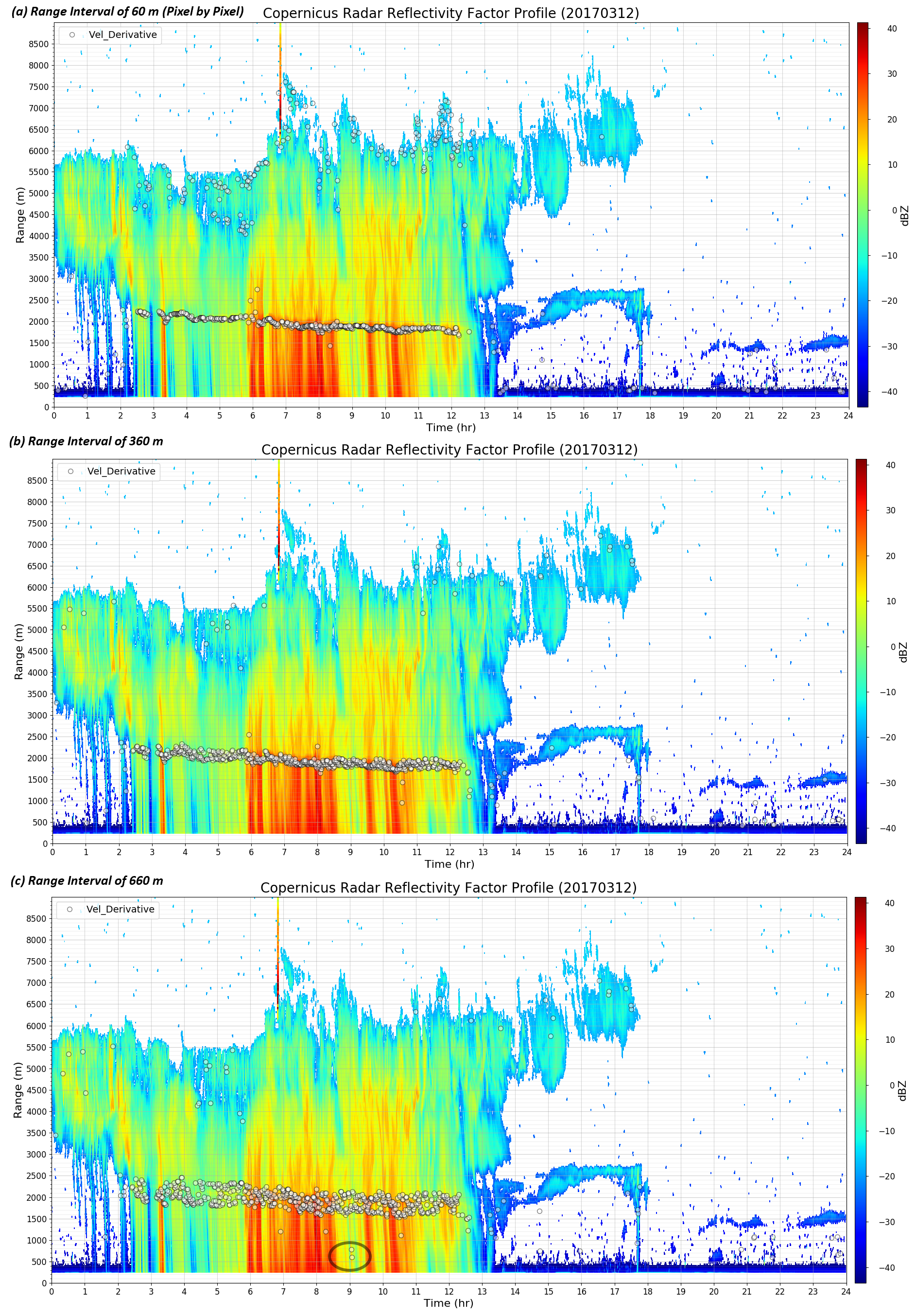
Figure 14: Bright band identified (white circles) by analysing the first derivative of the velocity with a range interval of 60 m (a), 360 m (b) and 660 m (c).
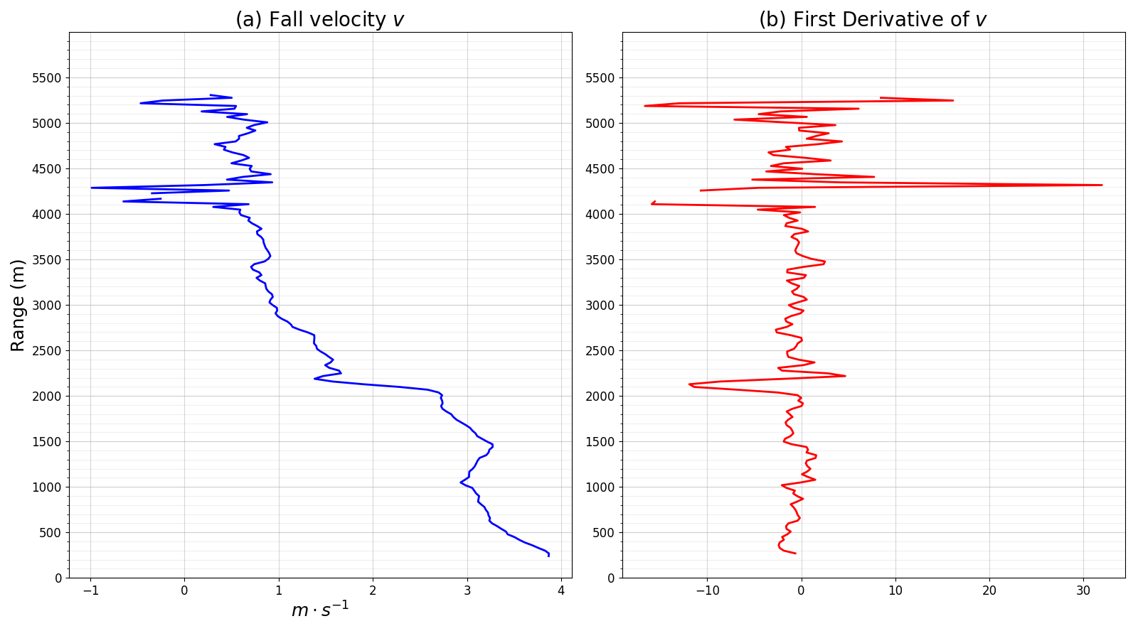
Figure 15: Vertical profiles of the Doppler velocity and its first derivative (60-m interval). The bright band should be located at where the first derivative is the smallest, but this identification is affected by noisy profiles above 4000 m.
As for analysing the bright band strength numerically, the ongoing method is to measure the “contrast of the image” – how well the bright band melting layer could be distinguishing from signals of non-melting precipitation. The hypothesis is that the stronger the bright band is, the stronger the contrast would be. More information about how to measure the image contrast can be found here. The contrast can be calculated using this equation:
where $I_{max}$ is the maximum intensity and $I_{min}$ is the minimum intensity. In the radar cases, $I_{max}$ is the maximum radar reflectivity factor ($dBZ_{max}$) and $I_{min}$ is the minimum radar reflectivity factor ($dBZ_{min}$). The region to calculate the contrast is the 750-m region with midpoint at where the bright band is detected by analysing the first derivative of velocity with a 360-m interval. For example, if the bright band height detected by the algorithm is 2000 m, then the region should be between 1625 m and 2375 m. The bright band width (BBW) is fixed instead of using the region identified by the Velocity Algorithm because the BBW analysed by the Velocity Algorithm could be variable, which introduces errors into the contrast calculation. Figure 16 shows the bright band detected and its strength (shown as the length of blue bars). It seems that there is an inversely proportional relationship between the “contrast” and the bright band strength. However, it is still an ongoing work to figure out the underlying relationship and whether there exists any other method to express the bright band strength more properly.

Figure 16: Bright band identified (white circles) by analysing the first derivative of the velocity with a range interval of 360 m. Blue bars show the "contrast" of the bright bands. The larger the contrast is, the longer the blue bars would be.