Auto-orthogonality can be extended to the more general case, where we require orthogonality between a function and one of its derivatives. We do not have a general prescription for their structure, but three example cases are given below.
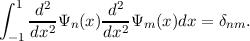
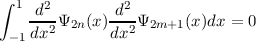
Consider a fourth order problem satisfying y(±1) = y′′(±1) = 0, where we attempt to construct a basis set whose second derivatives are orthogonal [3],
This may be motived by considering
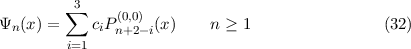
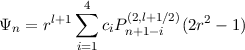
and integrating by parts twice. We find that the basis functions may be written
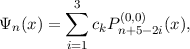 | (29) |
where, up to a normalization,
| c[1] | =  n(n + 1)(2n + 1), n(n + 1)(2n + 1), | ||
| c[2] | = -(2n + 3)(n2 + 3n + 5), | ||
| c[3] | =  (n + 2)(n + 3)(2n + 5). (n + 2)(n + 3)(2n + 5). |
Because of the symmetry of the original problem, each basis function is either even or odd and clearly
for any integer n and m, so that orthogonality between any such functions is automatic. Within each symmetry class, the matrices defined by
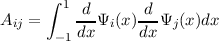 | (30) |
and
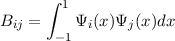 | (31) |
have much structure. The matrix A is tri-diagonal and the matrix B is penta-diagonal.
Additionally, note that the coefficients ci are proportional to [1,-2,1] in the limit n →∞. By applying both (5) and (6) (twice) to Pn(α,β)(x) we find that

Thus

as n →∞. Note that Jacobi polynomials are undefined with α,β taking non-positive integer values, since not only does their orthogonality relation break down but the 3-term recurrence relation fails as well. There is no contradiction here, since the equivalence is only true asymptotically and on the bulk of the interval and not within boundary layers.
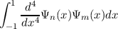
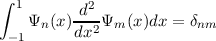
In the domain [-1,1], a basis set that satisfies
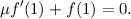
and the two boundary conditions
| μf′(1) + f(1) | = 0, | ||
| νf′(-1) + f(-1) | = 0, |
| c[1] | = μνn4 - 2n2μ - n2μν + 2n2ν - 4 | ||
| c[2] | = 2(ν + μ)(2n + 1) | ||
| c[3] | = -2ν + 2μ + 4 - 2nμν + 4nμ - 4nν - 5n2μν + 2n2μ - 2n2ν - 4n3μν - μνn4 | ||
Expressions for all quantities involved are provided below.
It is noteworthy that this sum of three Legendre polynomials is of the same form as that of the previous example.
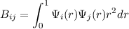
For this basis set, it is also of interest to look at the structure of the matrices defined by
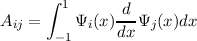 | (33) |
and
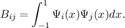 | (34) |
The matrix B turns out to be penta-diagonal, and A is upper triangular with a non-zero subdiagonal.
Additionally, note that the coefficients ci are proportional to [1,0,-1] in the limit n →∞. By applying both (5) and (6) to Pn(α,β)(x) we find that

Thus

as n →∞. Note that Jacobi polynomials with α = β = -1 are formally undefined (see comment above).
In spherical polar coordinates, a common spectral method is to expand in
terms of spherical harmonics in solid angle. The Laplacian operator,
∇2 =  +
+  +
+  , then becomes

where
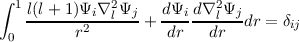
Additionally, regularity of a scalar implies that flm must behave as rl as r → 0 (see the introduction on regularity regarding this point). It is of interest to look for a regular basis set on the domain [0,1] that obeys the orthogonality condition
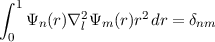
and a single first order boundary condition
The choice of the weight function r2 in the orthogonality relation is forced upon us. A basis set is

where, up to a normalization,
| c[1] | = (2l - 3 + 4n)(2l + 5 + 2n)(2l - 1 + 4n)(2nμl - μl + 1 + 2n2μ - μ - nμ)(2l + 3 + 2n) | ||
| c[2] | = -(2l - 3 + 4n)(2l + 3 + 2n)(2l + 3 + 4n)(2l + 1 + 2n)(-μl + 6nμl + 3 + nμ + 6n2μ + 2μ) | ||
| c[3] | = (2l - 1 + 4n)(2l + 5 + 4n)(2l + 1 + 2n)(-1 + 2l + 2n)(6nμl + μl + 5nμ + 3 + 3μ + 6n2μ) | ||
| c[4] | = -(2l - 3 + 2n)(2l + 5 + 4n)(2l + 3 + 4n)(-1 + 2l + 2n)(2nμl + μl + 3nμ + 2n2μ + 1) | ||
Expressions for all quantities involved are provided below.
For this basis set, it is also of note that the matrix defined by
 | (36) |
is tri-diagonal.
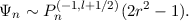
Additionally, note that the coefficients ci are proportional to [1,-3,3,-1] in the limit n →∞. By applying (5) to Pn(α,β)(x) we find that

Thus

as n →∞. Note that Jacobi polynomials with α = -1 are formally undefined. However, in this case (since β is a postive half integer) the 3-term recurrence relation still holds and they appear perfectly innocuous functions.
For the case of nonslip boundary conditions, the (unnormalised) basis is
with
| c1 | = (2l + 41)(2l + 27)(2l + 43)(2l + 25) | ||
| c2 | = -3(2l + 41)(2l + 25)(2l + 47)(2l + 23) | ||
| c3 | = 3(2l + 43)(2l + 49)(2l + 23)(21 + 2l) | ||
| c4 | = -(2l + 19)(2l + 49)(2l + 47)(21 + 2l) |
We now consider the orthogonality relation
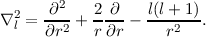
where ∇l2 =  -
- , which is motivated by rendering diagonal the
matrix
, which is motivated by rendering diagonal the
matrix
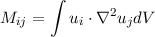
and expanding each mode ui in toroidal-poloidal decomposition and then in spherical harmonics.
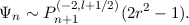
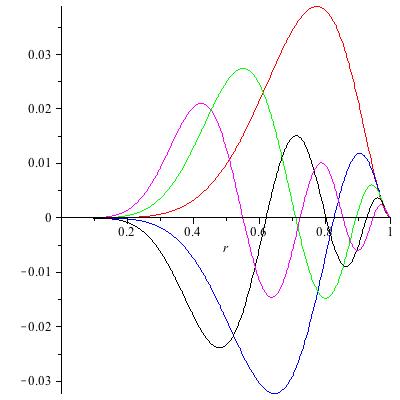
An orthogonal basis, satisfying Ψ(1) = Ψ′(1) = 0 is found to be
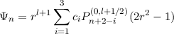
with
| c1 | = 2l + 4n + 1 | ||
| c2 | = -2(2l + 4n + 3) | ||
| c3 | = (2l + 4n + 5) |