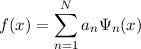
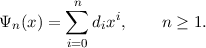
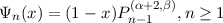
This online resource concerns the construction of a polynomial Galerkin basis {Ψn(x)}, each member of which satisfies two key properties (i) any given set of M homogeneous linear boundary conditions up to degree N - 1 and (ii) orthogonality to any other basis function. Although a brief overview of Galerkin methods — and the usage of this database — is provided below, far more detail regarding the theory and applications is contained in [2] and [3].
In the left hand frame of the page is listed a range of boundary conditions for (a) orthogonality in Cartesian coordinates, (b) orthogonality in polar geometries and (c) more general orthogonality relations involving derivatives. Common and physically motivated boundary conditions are given explicitly, followed by more general boundary conditions as far as the extent of computer algebra allows. Simply find the boundary condition of interest, and copy and paste the text defining the basis set. In the cases where α and β are unspecified, simply substitute your particular preference.
First published online 2009 at http://escholarship.org/uc/item/9vk1c6cm; updated Feb 2014.
Adopting a spectral method, or equivalently expanding an unknown function in terms a given basis {Ψn}
can be very helpful in solving, amongst others, partial differential equations, eigenvalue and variational problems. If each Ψn satisfies a prescribed set of linear and homogeneous boundary conditions, it follows simply that these same conditions are satisfied by f(x). If the expansion converges at a spectral or super-algebraic rate [1], then a severely truncated expansion may represent the function extremely well. In addition, the method of solution involves only finding the coefficients an; of particular note is that, for all intents and purposes, the boundary conditions may be ignored since they are already hard-wired into the numerical scheme.
One method of constructing a polynomial Galerkin basis set is the recombination of standard orthogonal polynomials [1]. However, such a basis set may be not only ill-conditioned, but in general will not inherit any of the optimal properties of the polynomials from which it was constructed. For instance,
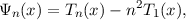
where Tn is a Chebyshev polynomial of the first kind, is a basis set suitable for representing all functions f for which f′(1) = 0. However, {Ψn(x)} is not orthogonal (by any useful definition) and has no optimal fitting properties (such as minimising the L∞ norm of the error as the Chebyshev polynomials themselves do). Furthermore, this basis set is very ill-conditioned as, when normalised, Ψn(x) →-x as n →∞ and so, for large n, all basis functions look the same.
A more general approach, in order to enforce orthogonality, is to adopt a Gram-Schmidt process. In the case of finding a set of polynomials that satisfy f′(1) = 0, we can write
Each coefficient di is determined by (i) the boundary condition Ψn′(1) = 0, (ii) orthogonality (by some definition) to each Ψj, j < n and (iii) a normalisation condition. However, this procedure has two major shortcomings. Firstly, in general, it requires symbolic calculation to determine the di. Adopting an integral measure of orthogonality, such as
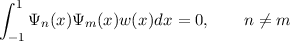
leads to di that, in general, grow extremely rapidly with n. This is an immediate consequence of the parsimonious representation of such a basis set in Jacobi polynomials whose monomial coefficients grow rapidly with n (see the discussion below). The only practical (and accurate) way of computing Ψn is by using computer algebra. Second, and most importantly, there is no way of knowing in advance what properties the basis functions, derived via the “black-box” Gram-Schmidt procedure, will have.
If the boundary conditions are sufficiently simple, for instance, f(1) = 0, we can write down an orthogonal basis set by exploiting properties of Jacobi polynomials. It may be written
 | (1) |
since Ψn(1) clearly vanishes and applying the standard orthogonality relation of Jacobi polynomials we see that

for some constants hn. For more complex boundary conditions, such as f′′(1) = 0 this approach is not possible.
Perhaps the simplest case with which to illustrate the concept of auto-orthogonality is the above basis
 | (2) |
that satisfies f(1) = 0. Using the standard index recurrence relations
 | (3) |
 | (4) |
 | (5) |
 | (6) |
we can write
 | (7) |
for coefficients ci(n), which take the (unnormalized) form
| c1(n) | = n(β + α + 2n)(α + β + n + 2), | ||
| c2(n) | = -(β + 1 + 2n + α)(2n2 + 2nβ + 2n + 2nα + βα + α2 + 3α + 2 + β), | ||
| c3(n) | = (α + n + 1)(β + n - 1)(β + α + 2n + 2), |
for n ≥ 2 and Ψ1(x) = 1 -x. Suppose we now consider constructing a basis set of the form
where Ψ1(x) = 1 - x and the ci are found using the three conditions
where w(x) = (1 - x)α(1 + x)β.
It must be that this new basis is the same that we have already found, namely Ψn(x) = (1 -x)Pn-1(α+2,β). It follows that the Ψn form an orthogonal set, even though we have only explicitly imposed that each is orthogonal to Ψ1. This property we term auto-orthogonality [3].
Note also that the ci take on the ratio [1,-2,1] as n →∞, a property that has great significance since the same asymptotic behavior arises from writing Pn(α,β)(x) in the form of (7) by applying (5) twice. It follows that

for large n.
This construction can be extended to the boundary condition f′(1) = 0. A basis set is
for any α > -1, β > -1 and where Pn(α,β)(x) is a Jacobi polynomial. The function Ψ1(x) = 1 is the lowest degree polynomial that satisfies the boundary condition. The three coefficients ci are determined by imposing
where w(x) = (1 - x)α(1 + x)β.
Remarkably, the {Ψn} are themselves orthogonal (auto-orthogonality)
The coefficients ci are (taking β = α)
| c1 | = 8α2 + 8n3α3 - 12n2α - 9n3α + 5n4α2 + 12n3α2 - 14nα3 - 27n2α2 + 2nα2 - 4n2α3 + n5α | ||
| + 10n4α + 2n5 + 4n2α4 - 8nα4 + 10α3 + 4α4 + 8nα + 2n - 4n3 + 2α | |||
| c2 | = -(2α4 + 6nα3 + 9α3 + 6n2α2 + 20nα2 + 14α2 + 2n3α + 15n2α + 19nα + 5α + 4n3 + 6n2 + 2n) | ||
| × (-1 + n2 - 2α + 2nα) | |||
| c3 | = -4n - α - 6n2 + 2n3 + 6n4 - α2 + α3 + 2n5 + α4 + 11nα3 + 2α5n + 8nα4 + 25n2α3 + 28n3α2 | ||
| + 13n4α + 9n3α3 + 5n4α2 + 26n2α2 - 11nα - 2nα2 + 22n3α + 7n2α4 + n5α |
Additional features of these auto-orthogonal sets are

For instance, if α = β = -1∕2, the {Ψn} behave like Chebyshev polynomials for large n and thus inherit their optimal characteristics.
We consider here a one-dimensional Cartesian domain (or one in which no further constraints are imposed on the functions apart from boundary conditions and smoothness). We will impose a given set of M homogeneous linear boundary conditions involving derivatives up to degree N - 1 at x = 1 only (hence the name “one-sided”). A basis set can be written
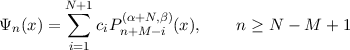
where the ci are found using
and Ψn,n = 1,2,…,N - M are computed using a Gram-Schmidt orthogonalisation procedure.
This basis set has the properties
The imposition of boundary conditions at x = -1 (only) requires a basis set of the form
where the ci are found as before.
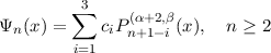
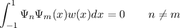
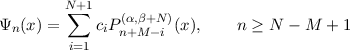
In the Cartesian domain [-1,1] we consider a basis set that satisfies any given set of M homogeneous linear boundary conditions up to degree N - 1 imposed at x = -1 or x = 1 (or both). It may be written
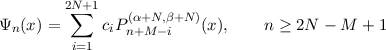
where the ci are found using
and Ψn,n = 1,2,…,2N -M are computed using a Gram-Schmidt orthogonalisation procedure.
The basis sets are found in various specific cases of the boundary conditions in section 3.
As in the one-sided case,
as n →∞.
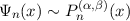
In polar geometries, due to the singularity of the coordinate system at the origin, expansions in radius (r) often require a regularity condition. This restricts the class of scalar functions within which the solution must lie to one of the form
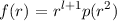
for some integer l and a function p. We assume this to be the case in what follows. In such a situation, we require a basis set that is of the above form and, in addition, satisfies M boundary conditions of maximum degree N - 1 at r = 1. It follows from the one-sided Cartesian case that such a basis can be written
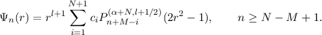
As before, the first few Ψn are determined using a Gram-Schmidt procedure. These satisfy the auto-orthogonality
and
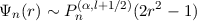
as n →∞.
There are two things of note. Firstly, the argument of the Jacobi polynomials is 2r2 - 1, mapping [0,1] → [-1,1] and rendering the Jacobi polynomial contribution an even function. Secondly, β is no longer free, being set to l + 1∕2. This ensures that the limiting behaviour of Pn(α,l+1∕2)(2r2 - 1) takes on the equal-ripple or equal-area property of the Chebyshev polynomials of the first and second kinds when α = -1∕2 or α = 1∕2 respectively. However, other choices of β are possible [4].
The basis sets are found in various specific cases of the boundary conditions in §4.
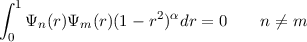
Making the functions orthogonal, as we have done, is transparently helpful for expansions of many kinds. But this is not always the best way to approach solutions of a differential equation as the resulting matrices may be full and poorly conditioned.
Given the developments so far, it is natural to ask if our algorithm can be extended, so that we impose orthogonality between, say, (d∕dx)kΨn(x) and (d∕dx)kΨm(x), or (d∕dx)kΨn(x) and Ψm(x), in place of that between Ψn and Ψm. For instance, if we were to solve the differential equation
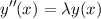
for an eigenvalue λ, this could be represented by the matrix problem
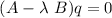
where we have written y(x) = ∑ iqiΨi(x) and
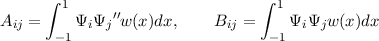
and q is a vector of the unknown spectral coefficients. If, for some choice of Ψ and weight function w(x), A and B could be made band-limited, then the numerical solution would be obtained expediently. In §6, we will give examples where A is diagonal. In general, the matrix B turns out to have significant structure, for instance, becoming either penta-diagonal or tri-diagonal.