In a full sphere geometry, the energy of a vector field over the unit sphere, written in toroidal-poloidal form and then decomposed into spherical harmonics, may be defined as the sum
where α indexes the spherical harmonics.
Auto-orthogonality can be extended to the case for which the basis functions
are
(i) regular at the origin
(ii) satisfy relevant boundary conditions at r = 1 and are
(iii) orthogonal with respect to the inner product defined for the toroidal or
poloidal scalars respectively
The toroidal component of a regular vector field that satisfies no particular boundary condition has an orthogonal basis of the form
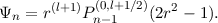
The toroidal component of a flow subject to nonslip boundary conditions, or the toroidal component of field in contact with an external electrical insulator simply satisfies regularity, T(1) = 0; an orthogonal basis is of the form

An alternative to the Worland polynomials [4] (which are orthogonal in a different norm) is the orthogonal basis set
for n ≥ 2.
The basis functions asymptotically collapse to a single family of one-sided Jacobi polynomials:

as n →∞.
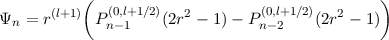
The poloidal component of a magnetic field in contact with an external electrical insulator satisfies regularity and (ii) S′(1) + lS(1) = 0 l ≥ 1 is the spherical harmonic degree. It has an orthogonal basis of the form

where
| c0 | = -2n2(l + 1) - n(l + 1)(2l - 1) - l(2l + 1) | ||
| c1 | = 2(l + 1)n2 + (2l + 3)(l + 1)n + (2l + 1)2 | ||
| c2 | = 4nl + l(2l + 1) |
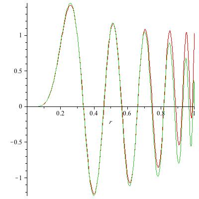
Distinct from most other closed form expressions for the basis functions given in [2; 3], this has a constant term, although scaling only linearly in n, compared to the Jacobi polynomial coefficients that scale quadratically. Note that the coefficients are in the ratio (1,-1,0) in the limit of large n, so that the basis functions asymptotically collapse to a single family of one-sided Jacobi polynomials:

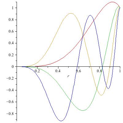
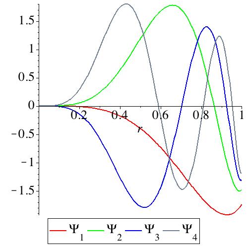
as n →∞. The figures below show some example basis functions and the asymptotic description of the 11th basis function.
The poloidal component of a nonslip flow satisfies regularity and S(1) = S′(1) = 0. Although an orthogonal basis can be written
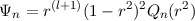
for some polynomial Qn, this has no [obvious] terse representation in terms of Jacobi polynomials. Instead, it may be written

where
| c0 | = 2n2 + (2l + 3)n | ||
| c1 | = -2n2 + (-7 - 2l)n - 2l - 5 | ||
| c2 | = 2l + 4n + 5 |
as n →∞.
A poloidal component of a flow satisfying a non-penetration condition at r = 1 satisfies S(1) = 0 and has an orthogonal basis of the form

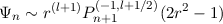
The poloidal component of a magnetic field which describes a purely radial field satisfies S′(1) = 0, and has an orthogonal basis of the form

where
| c0 | = -(2n - 1)(n + l) | ||
| c1 | = (2n + 1)(n + l + 1) |
Note that the coefficients are in the ratio (1,-1) in the limit of large n, so that the basis functions asymptotically collapse to a single family of one-sided Jacobi polynomials:

as n →∞.
In an electrical insulator defined in the region r > 1 an interior magnetic field may be extended as:

where the boundary condition
is satisfied. Noting that
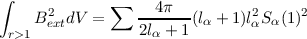
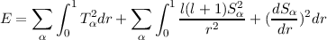
it follows that the total energy over all space of the poloidal magnetic field may be defined as the sum
![[ ∫ ]
∑ 4πlα(lα +-1) 1l(l +-1)S2α dS-α 2 2
E = 2lα + 1 r2 + ( dr ) dr + lαSα(1)
α 0](Galerkin92x.png)
where α indexes the harmonics.
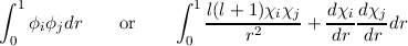
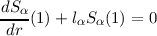
An orthogonal basis that satisfies the orthogonality
![∫ 1[l(l + 1)Ψn (r)Ψm (r) dΨn dΨm ]
---------2--------+ ---------dr + lΨn (1)Ψm (1) = δnm
0 r dr dr](Galerkin93x.png)
and the boundary condition S′(1) + lS(1) = 0 is of the form

Note that the coefficients are in the ratio (1,-1) in the limit of large n, so that the basis functions asymptotically collapse to a single family of one-sided Jacobi polynomials:

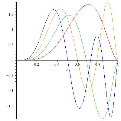
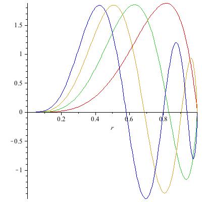
as n →∞. The figure shows some example basis functions normalised under the radial norm as defined above with l = 3.