|
|
SynFrac (v1.0)Generation of Synthetic Fracture
Patterns |
Purpose
This program can be used for creating synthetic rough fractures. Synthetic fractures is the term used to describe fractures that are created numerically in such a way that they share the same mean geometrical characteristics as specific natural fractures.
To create a synthetic fracture, set the parameters required and press the “Proceed” button in the program window. The creation process takes some time depending on the capabilities of the computer you use. After the fracture is synthesized you can view the result and save it for you own purposes.
Each fracture requires two random number seeds. These seeds do not refer to each surface. However the use of the same seeds will always give exactly the same fracture physically, and the fracture will have the parameters that you have set. In this way the program is purely deterministic. A suite of fractures that share the same physical parameters may be required e.g., for flow modelling. This can be achieved by retaining the same set parameters, and using several pairs of different random number seeds, one for each fracture required.
Parameters of Synthetic Fracture
 Using this panel you can choose one of the three methods, all of which
are based on spectral Fourier synthesis. The main idea exploited in these
methods is that the surfaces bounding the fracture should be similar at large
scale and relatively independent at micro-scale. As the degree of similarity
can be expressed through the correlation coefficient, so the difference between
these methods can be shown clearly by the behaviour of the correlation coefficient
for each method.
Using this panel you can choose one of the three methods, all of which
are based on spectral Fourier synthesis. The main idea exploited in these
methods is that the surfaces bounding the fracture should be similar at large
scale and relatively independent at micro-scale. As the degree of similarity
can be expressed through the correlation coefficient, so the difference between
these methods can be shown clearly by the behaviour of the correlation coefficient
for each method.
|
Brown (1995) |
|
|
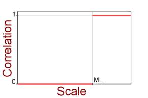
The method of S.R. Brown assumes the fracture surfaces to be perfectly matched at large scales and absolutely independent at small scales. The Mismatch Length (ML) separating these scales can be prescribed using the parameters panel. Beware that the abrupt discontinuity in correlation
is unphysical and can lead to underestimated apertures. However, this method
is the fastest to run. |
|
|
For more details about this method, refer to Brown, S.R. (1995) Simple mathematical model of
a rough fracture. Journal of Geophysical Research. 100, B4. |
|
|
Glover et al. (1998) |
|
|
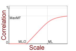
This method gives more physically reasonable synthetic fractures. Fracture surfaces are not perfectly correlated up to scale of the whole fracture pattern. The value of the Maximum Matching Fraction MaxMF can be prescribed using the parameters panel. Transition from small scale to large scale is smooth in contrast to the Brown method. While this method implements the smooth transition between matched and unmatched behaviour seen in real rock fractures (Glover et al, 1998b), it handles the mixing of particularly correlated random variables in a simple fashion that can lead to errors in the resulting fractures. |
|
|
For more details about this method, refer to Glover, P.W.J., Matsuki, K., Hikima R., Hayashi, K. (1998a) Synthetic rough fractures in rocks. Journal of Geophysical Research. 103, B5. Glover, P.W.J., Matsuki, K., Hikima R., Hayashi, K. (1998b) Fluid flow in synthetic rough fractures and application to the Hachimantai geothermal HDR test site. Journal of Geophysical Research. 103, B5. Glover, P.W.J., Matsuki, K., Hikima R., Hayashi,
K. (1999) Characterizing
rock fractures using synthetic fractal analogues.
Geothermal Sci. & Tech. 6. |
|
|
AUPG (2000) |
|
|
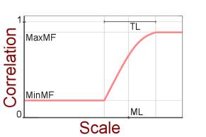
This new method was recently developed by the Aberdeen University Petrophysics Group and firstly implemented in the present software. It uses a generalized and improved approach of Brown and Glover et al. Both Minimum Matching Fraction (MinMF) and Maximum Matching Fraction (MaxMF) can be prescribed as well as the Transitional Length (TL) (see parameters panel description). The mathematics behind the method was also improved significantly. Specifically, the procedures for mixing partially correlated random variables had been made extremely robust. |
|
|
For more details about this method, refer to Ogilvie, S.R., Isakov, E. & Glover, P.W.J., Fluid flow through rough fractures. II: A new matching model for rough rock fractures, Earth Planet. Sci. Lett., 241, 454-465, 2006. |
|
Fracture Resolution
 Select a resolution for the synthetic fracture,
which is most appropriate for your aims. Smaller resolutions are faster to
implement.
Select a resolution for the synthetic fracture,
which is most appropriate for your aims. Smaller resolutions are faster to
implement.
Random Number Generator
 Choose one of the three high quality random
number generators. All these generators provide random sequences of sufficient
quality for the purpose of fracture synthesizing.
Choose one of the three high quality random
number generators. All these generators provide random sequences of sufficient
quality for the purpose of fracture synthesizing.
Choose two different numbers as a seeds for the
random sequences. Using these numbers again you can generate the same fracture
anytime (of course, other parameters should match as well). So you do not need
to store the large resulting files.
Hint: Large numbers consisting of odd digits
produce higher quality random numbers.
The random number generators were implemented
according to
Press, W.H., Teukolsky, S.A., Vetterling, W.T.,
Flannery, B.P. (1992) Numerical Recipes in C. Second Edition. Cambridge
University Press.
Parameters for the
Synthesizing Process
 Predefine these parameters of synthetic fracture
you need.
Predefine these parameters of synthetic fracture
you need.
Physical Size is the size of synthetic fracture to be created (in
millimetres).
Mismatch Length is the critical scale for the fracture surface forms (in
millimetres). See the Methods section for more
details.
Transitional Length is the difference between macro and micro scales (in
millimetres). This parameter is valid for the AUPG Method only and disabled for
other methods. See the Methods section for more
details.
Standard Deviation is the mean-square value of the fracture surface
deflections from the mean plane. The same value is applied to both fracture
surfaces in this version of the program.
Anisotropy Factor is used to generate anisotropic synthetic fractures. If
this value differs from unity, then all the scales in one direction along the
fracture surface will be greater than the scales in other direction. The same
value is applied to both fracture surfaces in this version of the program. The
fractal dimension of the surfaces is isotropic.
Fractal Dimension for each fracture surface is a value between 2 and 3,
which predetermines the roughness of the fracture surface. The same value is
applied to both surfaces in this version of the program.
Maximum Mismatch Fraction determines the required correlation between the
fracture surfaces at large scale. It varies from 0 to 1, where 1 represents
perfect matching at large scale (wavelength of the Fourier components) and 0
represents independency of the large-scale wavelength of the Fourier
components. This parameter is not used, and therefore is disabled in the Brown
Method. See the Methods section for more details.
Minimum Mismatch Fraction determines the required correlation between the
fracture surfaces in small-scale view. Again, this parameter varies from 0 to
1, where 0 represents independent behaviour of the fracture surfaces, and 1
represents perfectly matched behaviour. This parameter is valid for the AUPG
Method only and disabled for other methods. See the Methods
section for more details.
This panel allows you to view the map view and
profile views of the synthesized fracture. The main square field shows the map
view of the relief by the greyscale brightness variation (the lighter dots
correspond to higher elevation). You can use the View switch to observe top and
bottom surfaces of the fracture as well as the fracture aperture.
To observe a position where the fracture
surfaces touch, check the “Touch Point” box. A marker appears on the surface
map as a red square.
(Notice: the fracture surfaces may match
perfectly at some values of parameters. In this case all the surface points are
counted as touching. As a result you can observe fracture surface covered by
fine red mesh when the “Touch Point” box is checked.)
The relative vertical position of the fracture
surfaces is defined by arranging the surfaces to just touch at a single point.
By clicking on the main field of the map view,
you can choose a point to make cross-sections through the fracture surface. The
cross-section profiles appear by the sides of the main field of view. If you choose
a point on the top or bottom fracture surface then both cross-section profiles
will appear. Black and white lines correspond to the top and bottom surfaces
respectively. If you choose a point on the aperture view then only the aperture
profile will be shown.
Scales graded in mm are shown on both the
map-view and profile cross-sections. The mean arithmetic aperture of the whole
fracture and each of the current profiles are shown in the status bar at the
bottom of the window.
Press the “Save results” button if you want to
save the fracture data. Please refer to the Exchange
data section for further information about the file formats available.