5. Dispersion in Real Environments
The Gaussian plume equation, Eq. (47) is derived from Eq. (22) and this in
turn is only a true solution of the concentration equation, Eq. (21) if the
eddy diffusivities are constant. This is generally not true. For example,
in the neutrally stratified surface layer, the eddy viscosity  is given by
 and we can expect
 to behave similarly. In order to analyse
real environments we have at least 3 possibilities:
(i) Estimate (for example using surface layer theory) or measure
(usually indirectly by measuring wind fluctuations
to behave similarly. In order to analyse
real environments we have at least 3 possibilities:
(i) Estimate (for example using surface layer theory) or measure
(usually indirectly by measuring wind fluctuations
 and
and
 )
)
 ,
and then solve Eq. (21) numerically.
(ii) Assume that the solution (47) is still a reasonable approximation
but that the variation of
,
and then solve Eq. (21) numerically.
(ii) Assume that the solution (47) is still a reasonable approximation
but that the variation of  and
and  with
with  is different to
Eq. (48). Instead, we replace (48) by empirical relationships between
, and .
(iii) For some special cases, take
to vary with
is different to
Eq. (48). Instead, we replace (48) by empirical relationships between
, and .
(iii) For some special cases, take
to vary with  and solve
the concentration equation analytically.
and solve
the concentration equation analytically.
We now consider examples of (ii) and (iii).
5.1 Pasquill-Gifford Stability Classes
It is observed that in neutral stratification, Eq. (48) does not hold.
Instead, measurements suggest that and are proportional
to  for
for  in the range 0.75 to 1. This observation changes
when the atmospheric stability changes. For example, when the air is very
stable, vertical mixing is inhibited and grows only slowly with
. On the other hand, when there is strong solar heating of the surface,
there may be strong convective activity with large vertical motions; then
increases rapidly with .
in the range 0.75 to 1. This observation changes
when the atmospheric stability changes. For example, when the air is very
stable, vertical mixing is inhibited and grows only slowly with
. On the other hand, when there is strong solar heating of the surface,
there may be strong convective activity with large vertical motions; then
increases rapidly with .
Based on measurements of atmospheric turbulence over flat plains, Pasquill
and Gifford produced empirical results for the variation of and
with for six stability classes. These are shown in
Table 2.
truept
Guidelines are given for estimating the stability class from the wind
speed, cloud cover and time of day. These are given in Table 3.
truept
Figs. 9 and 10 show the variation of and with
for the six stability classes. These variations may be approximated by
and
where the constants  ,
,  ,
,  and
and  depend on the stability class as
shown in Table 4.
depend on the stability class as
shown in Table 4.
truept
With these values of and , the concentration can
be determined directly from Eq. (47). An example is shown in Fig. 11.
 =7.8
Fig. 9. Variation of with downwind distance
for the six Pasquill-Gifford stability classes.
=7.8
Fig. 9. Variation of with downwind distance
for the six Pasquill-Gifford stability classes.
Fig. 10. Variation of with downwind distance
for the six Pasquill-Gifford stability classes.
Fig. 11. The solution to the Gaussian plume equation
(47) with and given by the Pasquill-Gifford
recommendations for stability class C. Contours of concentration are shown
at  for a wind speed of 10 ms
 .
.
5.2 Dispersion from a Continuous Line Source
A major application here is to the dispersion of emissions from motor
vehicles travelling along a road on a cross-wind. If the wind is in the
-direction, perpendicular to the road, and  is along the road, then we
do not expect the concentration of pollutant to depend on . Just as
described in §4, we can neglect diffusion in the windward direction, so that
the concentration equation for a steady concentration distribution is
is along the road, then we
do not expect the concentration of pollutant to depend on . Just as
described in §4, we can neglect diffusion in the windward direction, so that
the concentration equation for a steady concentration distribution is
For neutral stability, it is reasonable to assume that
is equal to the
eddy viscosity in the neutral surface layer, so that
Therefore
We need also to describe the height variation of the wind,  . It would seem
to be consistent with the assumptions on
to take a logarithmic
velocity profile but unfortunately we cannot then solve Eq. (53) analytically.
Instead, a commonly made assumption is that
. It would seem
to be consistent with the assumptions on
to take a logarithmic
velocity profile but unfortunately we cannot then solve Eq. (53) analytically.
Instead, a commonly made assumption is that
where  is the wind speed at a fixed height
  . This can only be
approximately equal to the logarithmic profile (41) over a relatively
small height range. To get a reasonable correspondence, note that from Eq. (54)
. This can only be
approximately equal to the logarithmic profile (41) over a relatively
small height range. To get a reasonable correspondence, note that from Eq. (54)
and therefore
If we now substitute from Eq. (40) and (41) into the left and right sides of
the above equation, we get
and hence
Of course  should be a constant and so in Eq. (55) we take an average
value of over the range of interest. The precise value of should
really depend not only on the height range of interest but also on the
atmospheric stability. Generally, values in the range 0.1-0.4 are used, but
for high stability they may be even larger. Typical values are given in
Table 5.
should be a constant and so in Eq. (55) we take an average
value of over the range of interest. The precise value of should
really depend not only on the height range of interest but also on the
atmospheric stability. Generally, values in the range 0.1-0.4 are used, but
for high stability they may be even larger. Typical values are given in
Table 5.
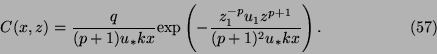
Using Eq. (54), Eq. (53) becomes
and the solution is
Note that the concentration at the ground decreases with like  ,
unlike the one-dimensional diffusion solution with constant diffusivity
which suggests decay like
,
unlike the one-dimensional diffusion solution with constant diffusivity
which suggests decay like  . Note also that the decay rate is
larger for smaller , i.e. for unstable air flow. Eq. (57) has been shown
to agree quite well with observations.
. Note also that the decay rate is
larger for smaller , i.e. for unstable air flow. Eq. (57) has been shown
to agree quite well with observations.
back to syllabus